Tutorial¶

Getting started¶

Import library and packages¶

[1]:

import os
import sys
root_folder = os.path.dirname(os.getcwd())
sys.path.append(root_folder)
import ResoFit
from ResoFit.calibration import Calibration
from ResoFit.fitresonance import FitResonance
from ResoFit.experiment import Experiment
from ResoFit._utilities import Layer
import numpy as np
import matplotlib.pyplot as plt

Global paramters¶

min energy of 7 eV (has to be greater than 1 x 10-5 eV)
max energy of 150 eV (has to be less than 3000 eV)
energy steps to interpolate database: 0.1 eV

[2]:

energy_min = 7
energy_max = 150
energy_step = 0.01

File locations¶

data/* (directory to locate the file)
data_file (YOUR_DATA_FILE.txt or .csv)
spectra_file (YOUR_SPECTRA_FILE.txt or .csv)

[3]:

folder = 'data/_data_for_tutorial'
data_file = 'raw_data.csv'
spectra_file = 'spectra.txt'

Preview data using Experiment()¶

Note this is meant to demenstrate the functionality of Experiment() class. These operations are not needed for general calibration and fitting.

Data¶

Values are in transmission with image number as indexes after extracting with ImageJ

[5]:

experiment.data

[5]:

	0
0	1.025803
1	1.027222
2	1.029864
3	1.029095
4	1.032496
5	1.038683
6	1.042255
7	1.041075
8	1.034811
9	1.031851
10	1.032940
11	1.032937
12	1.034382
13	1.034205
14	1.035444
15	1.033757
16	1.039690
17	1.043947
18	1.043075
19	1.039344
20	1.039744
21	1.041730
22	1.041170
23	1.042075
24	1.040100
25	1.039565
26	1.039670
27	1.041171
28	1.044951
29	1.044430
...	...
2776	0.915787
2777	0.920761
2778	0.921717
2779	0.930883
2780	0.923302
2781	0.923815
2782	0.924068
2783	0.916594
2784	0.914615
2785	0.919048
2786	0.924325
2787	0.923643
2788	0.920561
2789	0.920570
2790	0.923603
2791	0.919968
2792	0.916965
2793	0.926718
2794	0.925573
2795	0.919824
2796	0.920326
2797	0.920852
2798	0.928154
2799	0.918875
2800	0.919932
2801	0.917441
2802	0.915185
2803	0.919612
2804	0.921282
2805	0.905286

2806 rows × 1 columns

Spectra¶

Column 0 time values (seconds) with image number as indexes
Column 1 neutron counts

[6]:

experiment.spectra

[6]:

	0	1
0	9.600000e-07	22192427
1	1.120000e-06	20966591
2	1.280000e-06	19678909
3	1.440000e-06	19890967
4	1.600000e-06	20968632
5	1.760000e-06	21026731
6	1.920000e-06	20464927
7	2.080000e-06	21112328
8	2.240000e-06	22520473
9	2.400000e-06	22849349
10	2.560000e-06	22234183
11	2.720000e-06	21483270
12	2.880000e-06	20741476
13	3.040000e-06	20045837
14	3.200000e-06	19278237
15	3.360000e-06	18293220
16	3.520000e-06	17256754
17	3.680000e-06	16811295
18	3.840000e-06	17305194
19	4.000000e-06	18163422
20	4.160000e-06	18526230
21	4.320000e-06	18573412
22	4.480000e-06	18822753
23	4.640000e-06	18829949
24	4.800000e-06	18510897
25	4.960000e-06	18082372
26	5.120000e-06	17696805
27	5.280000e-06	17336846
28	5.440000e-06	16983927
29	5.600000e-06	16640908
...	...	...
2776	4.451200e-04	2467945
2777	4.452800e-04	2466877
2778	4.454400e-04	2469613
2779	4.456000e-04	2468271
2780	4.457600e-04	2471169
2781	4.459200e-04	2471734
2782	4.460800e-04	2466328
2783	4.462400e-04	2469199
2784	4.464000e-04	2466776
2785	4.465600e-04	2466053
2786	4.467200e-04	2476433
2787	4.468800e-04	2474714
2788	4.470400e-04	2469559
2789	4.472000e-04	2474567
2790	4.473600e-04	2471115
2791	4.475200e-04	2472997
2792	4.476800e-04	2476153
2793	4.478400e-04	2478613
2794	4.480000e-04	2474287
2795	4.481600e-04	2475409
2796	4.483200e-04	2478018
2797	4.484800e-04	2481255
2798	4.486400e-04	2484636
2799	4.488000e-04	2493780
2800	4.489600e-04	2499320
2801	4.491200e-04	2499035
2802	4.492800e-04	2509962
2803	4.494400e-04	2502085
2804	4.496000e-04	2488273
2805	4.497600e-04	11391066

2806 rows × 2 columns

Remove unwanted data points¶

[7]:

experiment.slice(slice_start=3, slice_end=2801, reset_index=False)

[7]:

(3       0.000001
 4       0.000002
 5       0.000002
 6       0.000002
 7       0.000002
 8       0.000002
 9       0.000002
 10      0.000003
 11      0.000003
 12      0.000003
 13      0.000003
 14      0.000003
 15      0.000003
 16      0.000004
 17      0.000004
 18      0.000004
 19      0.000004
 20      0.000004
 21      0.000004
 22      0.000004
 23      0.000005
 24      0.000005
 25      0.000005
 26      0.000005
 27      0.000005
 28      0.000005
 29      0.000006
 30      0.000006
 31      0.000006
 32      0.000006
           ...
 2771    0.000444
 2772    0.000444
 2773    0.000445
 2774    0.000445
 2775    0.000445
 2776    0.000445
 2777    0.000445
 2778    0.000445
 2779    0.000446
 2780    0.000446
 2781    0.000446
 2782    0.000446
 2783    0.000446
 2784    0.000446
 2785    0.000447
 2786    0.000447
 2787    0.000447
 2788    0.000447
 2789    0.000447
 2790    0.000447
 2791    0.000448
 2792    0.000448
 2793    0.000448
 2794    0.000448
 2795    0.000448
 2796    0.000448
 2797    0.000448
 2798    0.000449
 2799    0.000449
 2800    0.000449
 Name: 0, Length: 2798, dtype: float64, 3       1.029095
 4       1.032496
 5       1.038683
 6       1.042255
 7       1.041075
 8       1.034811
 9       1.031851
 10      1.032940
 11      1.032937
 12      1.034382
 13      1.034205
 14      1.035444
 15      1.033757
 16      1.039690
 17      1.043947
 18      1.043075
 19      1.039344
 20      1.039744
 21      1.041730
 22      1.041170
 23      1.042075
 24      1.040100
 25      1.039565
 26      1.039670
 27      1.041171
 28      1.044951
 29      1.044430
 30      1.044017
 31      1.045077
 32      1.042383
           ...
 2771    0.937393
 2772    0.927724
 2773    0.921393
 2774    0.931766
 2775    0.930592
 2776    0.915787
 2777    0.920761
 2778    0.921717
 2779    0.930883
 2780    0.923302
 2781    0.923815
 2782    0.924068
 2783    0.916594
 2784    0.914615
 2785    0.919048
 2786    0.924325
 2787    0.923643
 2788    0.920561
 2789    0.920570
 2790    0.923603
 2791    0.919968
 2792    0.916965
 2793    0.926718
 2794    0.925573
 2795    0.919824
 2796    0.920326
 2797    0.920852
 2798    0.928154
 2799    0.918875
 2800    0.919932
 Name: 0, Length: 2798, dtype: float64)

Retrieve values for X-axis¶

In ‘neutron energy’¶

[8]:

experiment.x_raw(offset_us=0., source_to_detector_m=16)

[8]:

array([  6.45188613e+05,   5.22602776e+05,   4.31903121e+05, ...,
         6.64684718e+00,   6.64210874e+00,   6.63737536e+00])

In ‘neutron wavelength’¶

[9]:

experiment.x_raw(angstrom=True, offset_us=0., source_to_detector_m=16)

[9]:

array([ 0.00035604,  0.0003956 ,  0.00043516, ...,  0.11092624,
        0.1109658 ,  0.11100536])

Retrieve values for Y-axis¶

In ‘neutron attenuation’¶

[10]:

experiment.y_raw()

[10]:

array([-0.029095, -0.032496, -0.038683, ...,  0.071846,  0.081125,
        0.080068])

In ‘neutron transmission’¶

[11]:

experiment.y_raw(transmission=True)

[11]:

array([ 1.029095,  1.032496,  1.038683, ...,  0.928154,  0.918875,
        0.919932])

In ‘neutron attenuation’ & remove baseline¶

[12]:

experiment.y_raw(baseline=True)

[12]:

array([ 0.0183733 ,  0.01488139,  0.00860353, ...,  0.01160011,
        0.02088986,  0.01984365])

Retrieve interpolated values for both X-axis & Y-axis¶

X-axis: ‘neutron energy’

Y-axis: ‘neutron attenuation’

[13]:

experiment.xy_scaled(energy_min=energy_min, energy_max=energy_max, energy_step=energy_step,
                     angstrom=False, transmission=False,
                     offset_us=0, source_to_detector_m=15,
                     baseline=True)

[13]:

(array([   7.  ,    7.01,    7.02, ...,  149.98,  149.99,  150.  ]),
 array([ 0.00584673, -0.00275185,  0.00486153, ...,  0.01071007,
         0.01063659,  0.01056193]))

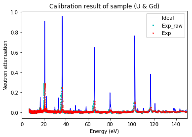
Plot raw in various ways¶

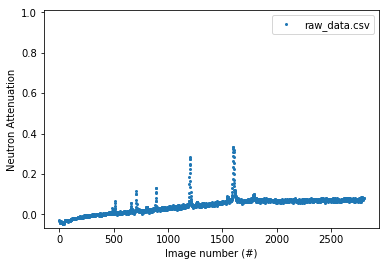
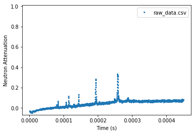
Attenuation vs. image number¶

[14]:

experiment.plot_raw(x_axis='number')
plt.show()

Attenuation vs. recorded time¶

Parameters need to be specified: - time_unit from ['s', 'us', 'ns']. (‘us’) is default

[15]:

experiment.plot_raw(x_axis='time')
plt.show()

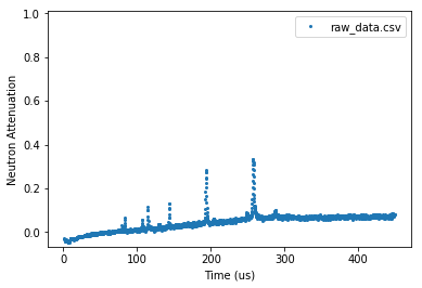
[16]:

experiment.plot_raw(x_axis='time', time_unit='s')
plt.show()

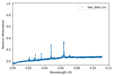
Attenuation vs. neutron wavelength¶

Parameters need to be specified: - lambda_xmax in (angstrom) - offset_us in (us) - source_to_detector_m in (m)

[17]:

experiment.plot_raw(x_axis='lambda', lambda_xmax=0.12,
                   offset_us=0, source_to_detector_m=16)
plt.show()

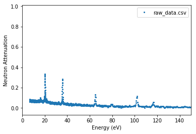
Attenuation vs. neutron energy¶

Parameters need to be specified: - energy_xmax in (eV) - offset_us in (us) - source_to_detector_m in (m)

[18]:

experiment.plot_raw(x_axis='energy', energy_xmax=150,
                    offset_us=0, source_to_detector_m=16)
plt.show()

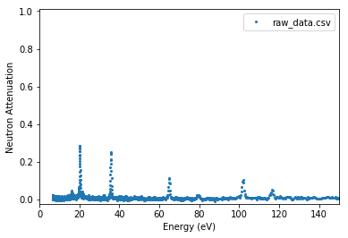
Remove baseline for plot¶

Note: this only changes the display of data, not the data values.

[19]:

experiment.plot_raw(offset_us=0, source_to_detector_m=16,
                    x_axis='energy', baseline=True,
                    energy_xmax=150)
plt.show()

Operation to experiment data¶

experiment.norm_to(file=background.csv)

This can be used to further normalize signal. (data divide background)

Note: this will change the data values.

Input sample info¶

Gd and U mixed foil
thickness neutron path within the sample in (mm)
density sample density in (g/cm3), if omitted, pure solid density will be used in fitting
repeat : reptition number if the data is summed of multiple runs (default: 1)

[20]:

layer_1 = 'U'
thickness_1 = 0.05 # mm
density_1 = None # g/cm^3 (if None or omitted, pure solid density will be used in fitting step)
layer_2 = 'Gd'
thickness_2 = 0.05 # mm
density_2 = None # g/cm^3 (if None or omitted, pure solid density will be used in fitting step)

Create sample layer

Note: Input each element as single layer.

[21]:

layer = Layer()
layer.add_layer(layer=layer_1, thickness_mm=thickness_1, density_gcm3=density_1)
layer.add_layer(layer=layer_2, thickness_mm=thickness_2, density_gcm3=density_2)

Calibration¶

Estimated intrumental parameters¶

input estimated source to detector distance (m)
input estimated possible time offset in spectra file (us)

Note: a separated Experiment() will be created after the initialization of Calibration(). Calibration.slice() is needed if you would like to remove unwanted data points by indexes.

[22]:

source_to_detector_m = 16.
offset_us = 0

Class initialization¶

Pass all the parameters definded above into the Calibration()

[23]:

calibration = Calibration(data_file=data_file,
                          spectra_file=spectra_file,
                          raw_layer=layer,
                          energy_min=energy_min,
                          energy_max=energy_max,
                          energy_step=energy_step,
                          folder=folder,
                          baseline=True)

Equations for (time-wavelength-energy) conversion¶

\[E = \frac {81.787 }{ \lambda^2 }\]

\(E\) : energy in (meV),

\(\lambda\) : wavelength in (Å).

\[\lambda = 0.3956\frac{t_{record} + t_{offset}}{L}\]

\(t_{record}\) : recorded time in (µs),

\(t_{offset}\) : recorded time offset in (µs),

\(L\) : source to detector distance in (cm).

Calibrate instrumental parameters¶

using source_to_detector_m or offset_us or both to minimize the difference between the measured resonance signals and the simulated resonance signals from ImagingReso within the range specified in global parameters
vary can be one of [‘source_to_detector’, ‘offset’, ‘all’] (default is ‘all’)
fitting parameters are displayed

[24]:

calibration.calibrate(source_to_detector_m=source_to_detector_m,
                      offset_us=offset_us,
                      vary='all')

-------Calibration-------
Params before:
Name                     Value      Min      Max   Stderr     Vary     Expr Brute_Step
offset_us                    0     -inf      inf     None     True     None     None
source_to_detector_m        16     -inf      inf     None     True     None     None
Params after:
Name                     Value      Min      Max   Stderr     Vary     Expr Brute_Step
offset_us                2.755     -inf      inf  0.03047     True     None     None
source_to_detector_m     16.44     -inf      inf 0.002896     True     None     None
Calibration chi^2 : 51.508119690122165

[24]:

<lmfit.minimizer.MinimizerResult at 0x119da62b0>

Retrieve calibrated parameters¶

[25]:

calibration.calibrated_offset_us

[25]:

2.754524867719895

[26]:

calibration.calibrated_source_to_detector_m

[26]:

16.437347811454231

Plot calibration result¶

using the best fitted source_to_detector_m and offset_us to show the calibrated resonance signals from measured data and the expected resonance positions from ImagingReso
measured data before and after is ploted with raw data points instead of interpolated data points. However, the interpolated data was used during the calibration step above.

Default layout¶

[27]:

calibration.plot()

Hide table¶

[28]:

calibration.plot(table=False)

Hide grid¶

[29]:

calibration.plot(table=False, grid=False)

Plot before to compare¶

[30]:

calibration.plot(table=False, grid=False, before=True)

Show all elements¶

[31]:

calibration.plot(table=False, grid=False, all_elements=True)

Show all isotopes¶

[32]:

calibration.plot(table=False, grid=False, all_isotopes=True)

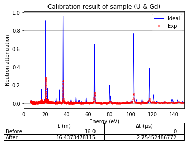
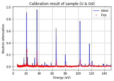
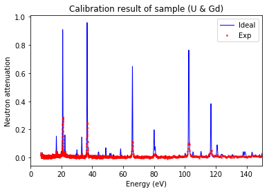
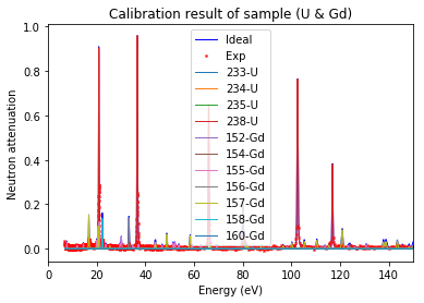
Show specified items¶

Format as list with each name in string

[33]:

calibration.plot(table=False, grid=False, items_to_plot=['U', 'U-238', 'Gd-156'])

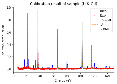
Note: 'U*' can be used to represent all the isotopes of uranium

[34]:

calibration.plot(table=False, grid=False, items_to_plot=['U', 'U*', 'Gd-156'])

Fit resonances¶

Class initialization¶

Pass all the parameters definded and calibrated into the FitResonance()

[35]:

fit = FitResonance(spectra_file=spectra_file,
                   data_file=data_file,
                   folder=folder,
                   energy_min=energy_min,
                   energy_max=energy_max,
                   energy_step=energy_step,
                   calibrated_offset_us=calibration.calibrated_offset_us,
                   calibrated_source_to_detector_m=calibration.calibrated_source_to_detector_m,
                   baseline=True)

Fitting equations¶

Beer-Lambert Law:¶

\[T\left( E \right) =\frac { I\left( E \right) }{ { I }_{ 0 }\left( E \right) } =exp\left[ -\sum\nolimits_i { { N }_{ i }{ d }_{ i } } \sum\nolimits_j { { \sigma }_{ ij }\left( E \right) { A }_{ ij } } \right]\]

\({ N }_{ i }\) : number of atoms per unit volume of element \(i\),

\({ d }_{ i }\) : effective thickness along the neutron path of element \(i\),

\({ \sigma }_{ ij }\left( E \right)\) : energy-dependent neutron total cross-section for the isotope \(j\) of element \(i\),

\({ A }_{ ij }\) : abundance for the isotope \(j\) of element \(i\).

\[{N_i} = {N_A}{C_i} = \frac { {N_A}{\rho_i}} {\sum\nolimits_j {m_{ij}{A_{ij}}}}\]

\({N_A}\) : Avogadro’s number,

\({C_i}\) : molar concentration of element \(i\),

\({\rho_i}\) : density of the element \(i\),

\(m_{ij}\) : atomic mass values for the isotope \(j\) of element \(i\).

How to fit the resonance signals¶

using thickness (mm) or density (g/cm3) to minimize the difference between the measured resonance signals and the simulated resonance signals from ImagingReso within the range specified in global parameters
vary can be one of [‘thickness’, ‘density’] (default is ‘density’)
fitting parameters are displayed

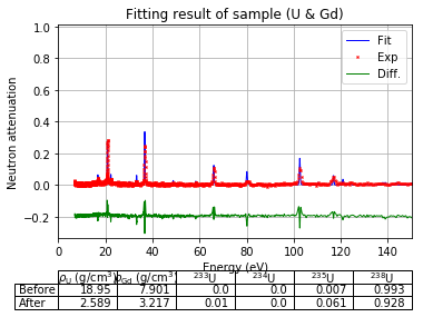
[36]:

fit_result = fit.fit(layer, vary='density')

-------Fitting (density)-------
Params before:
Name                Value      Min      Max   Stderr     Vary     Expr Brute_Step
density_gcm3_Gd     7.901        0      inf     None     True     None     None
density_gcm3_U      18.95        0      inf     None     True     None     None
thickness_mm_Gd      0.05        0      inf     None    False     None     None
thickness_mm_U       0.05        0      inf     None    False     None     None
Params after:
Name                Value      Min      Max   Stderr     Vary     Expr Brute_Step
density_gcm3_Gd     3.217        0      inf  0.04812     True     None     None
density_gcm3_U      2.589        0      inf  0.01818     True     None     None
thickness_mm_Gd      0.05        0      inf        0    False     None     None
thickness_mm_U       0.05        0      inf        0    False     None     None
Fitting chi^2 : 2.7164917570446554

Output fitted result in molar concentration¶

unit: mol/cm3

[37]:

fit.molar_conc()

Molar-conc. (mol/cm3)   Before_fit      After_fit
U       0.07961217820137899     0.010874916048358519
Gd      0.05024483306836248     0.020460587861440557

[37]:

{'Gd': {'density': {'units': 'g/cm3', 'value': 3.2174274412115276},
  'layer': 'Gd',
  'molar_conc': {'units': 'mol/cm3', 'value': 0.020460587861440557},
  'molar_mass': {'units': 'g/mol', 'value': 157.25},
  'thickness': {'units': 'mm', 'value': 0.05}},
 'U': {'density': {'units': 'g/cm3', 'value': 2.5885444133322855},
  'layer': 'U',
  'molar_conc': {'units': 'mol/cm3', 'value': 0.010874916048358519},
  'molar_mass': {'units': 'g/mol', 'value': 238.02891},
  'thickness': {'units': 'mm', 'value': 0.05}}}

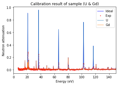
Plot fitting result¶

using the best fitted density to show the measured resonance signals and the fitted resonance signals from ImagingReso
measured data before and after is ploted with raw data points instead of interpolated data points. However, the interpolated data was used during the fitting step above.

Default layout¶

[38]:

fit.plot()

Hide difference plot¶

[39]:

fit.plot(error=False)

Hide table¶

[40]:

fit.plot(table=False)

Hide grid & show before¶

[41]:

fit.plot(table=False, grid=False, before=True)

Show all elements¶

[42]:

fit.plot(table=False, grid=False, all_elements=True)

Show all isotopes¶

[43]:

fit.plot(table=False, grid=False, all_isotopes=True)

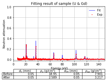
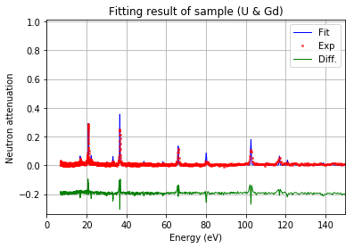
Show specified items¶

Format as list with each name in string

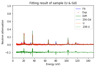
[44]:

fit.plot(table=False, grid=False, items_to_plot=['U', 'U-238', 'Gd-156'])

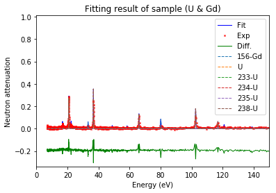
[45]:

fit.plot(table=False, grid=False, items_to_plot=['U', 'U*', 'Gd-156'])

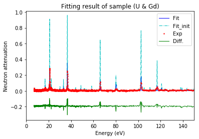
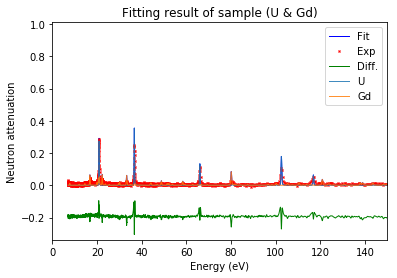
Fit isotopic ratios¶

specify the element you would like to perform isotopic (by at.%) fitting.

Note: Processing time of this step might be long.

[46]:

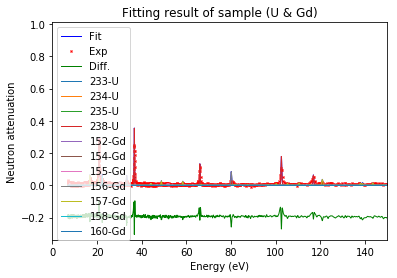
fit.fit_iso(layer='U')

-------Fitting (isotopic at.%)-------
Params before:
Name     Value      Min      Max   Stderr     Vary     Expr Brute_Step
U233         0        0        1     None     True     None     None
U234   5.5e-05        0        1     None     True     None     None
U235    0.0072        0        1     None     True     None     None
U238    0.9927        0        1     None    False 1-U233-U234-U235     None
Params after:
Name     Value      Min      Max   Stderr     Vary     Expr Brute_Step
U233    0.0101        0        1  0.03743     True     None     None
U234  5.316e-06        0        1  0.04623     True     None     None
U235   0.06146        0        1  0.03617     True     None     None
U238    0.9284        0        1  0.05946    False 1-U233-U234-U235     None
Fit iso chi^2 : 2.700599444474776

[47]:

fit.molar_conc()

Molar-conc. (mol/cm3)   Before_fit      After_fit
U       0.07968367366422123     0.01088468223204817
Gd      0.05024483306836248     0.020460587861440557

[47]:

{'Gd': {'density': {'units': 'g/cm3', 'value': 3.2174274412115276},
  'layer': 'Gd',
  'molar_conc': {'units': 'mol/cm3', 'value': 0.020460587861440557},
  'molar_mass': {'units': 'g/mol', 'value': 157.25},
  'thickness': {'units': 'mm', 'value': 0.05}},
 'U': {'density': {'units': 'g/cm3', 'value': 2.5885444133322855},
  'layer': 'U',
  'molar_conc': {'units': 'mol/cm3', 'value': 0.01088468223204817},
  'molar_mass': {'units': 'g/mol', 'value': 237.81534069141117},
  'thickness': {'units': 'mm', 'value': 0.05}}}

[48]:

fit.plot()

Tutorial¶

Getting started¶

Import library and packages¶

Global paramters¶

File locations¶

Preview data using Experiment()¶

Load the related files into Experiment()¶

Data¶

Spectra¶

Remove unwanted data points¶

Retrieve values for X-axis¶

In ‘neutron energy’¶

In ‘neutron wavelength’¶

Retrieve values for Y-axis¶

In ‘neutron attenuation’¶

In ‘neutron transmission’¶

In ‘neutron attenuation’ & remove baseline¶

Retrieve interpolated values for both X-axis & Y-axis¶

Plot raw in various ways¶

Attenuation vs. image number¶

Attenuation vs. recorded time¶

Attenuation vs. neutron wavelength¶

Attenuation vs. neutron energy¶

Remove baseline for plot¶

Operation to experiment data¶

Input sample info¶

Calibration¶

Estimated intrumental parameters¶

Class initialization¶

Equations for (time-wavelength-energy) conversion¶

Calibrate instrumental parameters¶

Retrieve calibrated parameters¶

Plot calibration result¶

Default layout¶

Hide table¶

Hide grid¶

Plot before to compare¶

Show all elements¶

Show all isotopes¶

Show specified items¶

Fit resonances¶

Class initialization¶

Fitting equations¶

Beer-Lambert Law:¶

How to fit the resonance signals¶

Output fitted result in molar concentration¶

Plot fitting result¶

Default layout¶

Hide difference plot¶

Hide table¶

Hide grid & show before¶

Show all elements¶

Show all isotopes¶

Show specified items¶

Fit isotopic ratios¶